4. Predictive Tool
4.1. Currently Supported Models
4.1.1. AGCRN
AGCRN (Adaptive Graph Convolutional Recurrent Network) is a deep nerual network for traffic prediction consisting of two adaptive module and recurrent networks.
- Reference Paper:
- Reference Implementation:
4.1.2. ARIMA
ARIMA (Autoregressive Integrated Moving Average) is a widely used classical statistical model on time series prediction.
- Reference Paper:
- Reference Package:
pandas,statsmodels
4.1.3. ASTGCN
ASTGCN (Attenion Based Spatial-temporal Graph Convolutional Networks) is a deep neural network for traffic flow forecasting. It models temporal-dependencies from three perspectives using attetion mechanism. And it models spatial-dependencies employing graph convolutions.
4.1.4. DCRNN
DCRNN (Diffusion Convolutional Recurrent Neural Network) is a deep learning framework for traffic forecasting that incorporates both spatial and temporal dependency in the traffic flow. It captures the spatial dependency using bidirectional random walks on the graph, and the temporal dependency using the encoder-decoder architecture with scheduled sampling.
4.1.5. DeepST
DeepST (Deep learning-based prediction model for Spatial-Temporal data) is composed of three components: 1) temporal dependent instances: describing temporal closeness, period and seasonal trend; 2) convolutional neural networks: capturing near and far spatial dependencies; 3) early and late fusions: fusing similar and different domains' data.
4.1.6. GeoMAN
GeoMAN (Multi-level Attention Networks for Geo-sensory Time Series Prediction) consists of two major parts: 1) A multi-level attention mechanism (including both local and global spatial attentions in encoder and temporal attention in decoder) to model the dynamic spatio-temporal dependencies; 2) A general fusion module to incorporate the external factors from different domains (e.g., meteorology, time of day and land use).
4.1.7. GMAN
GMAN (Graph Multi-Attention Network) is a deep nerual network for traffic prediction adopting encoder-decoder architecture. Both encode and decoder consist of multiple spatio-temporal attention blocks to model spatio-temporal dependencies.
- Reference Paper:
- Reference Implementation:
4.1.8. GraphWaveNet
GraphWaveNet is an end-to-end novel graph neural network. It captures spatial dependencies through a self-adptive adjacency matrix. And it captures temporal dependencies through convolutions.
- Reference Paper:
- Reference Implementation:
4.1.9. HM (Historical Mean)
HM is a constant model and always forecasts the sample mean of the historical data.
4.1.11. STGCN
STGCN (Spatio-temporal Graph Convolutional Networks) is a deep learning framework for traffic forecasting with complete convolutional structures.
- Reference Paper:
- Reference Implementation:
4.1.12. STMeta
STMeta is our prediction model, which requires extra graph information as input, and combines Graph Convolution LSTM and Attention mechanism.
- Reference Package:
tensorflow
4.1.13. ST-MGCN
ST-MGCN (Spatiotemporal Multi-graph Convolution Network) is a deep learning based model which encoded the non-Euclidean correlations among regions using multiple graphs and explicitly captured them using multi-graph convolution.
4.1.14. ST-ResNet
ST-ResNet is a deep-learning model with an end-to-end structure based on unique properties of spatio-temporal data making use of convolution and residual units.
- Reference Paper:
- Reference Implementation:
4.1.15. STSGCN
STSGCN (Spatial-temporal Synchronous Graph Convolutional Networks) is a deep learning framework for spatial-temporal network data forecasting. It is able to capture spatial-temporal dependencies through a designed spatial-temporal synchronous modeling mechanism.
4.1.16. XGBoost
XGBoost is a gradient boosting machine learning algorithm widely used in flow prediction and other machine learning prediction areas.
- Reference Paper:
- Reference Package:
xgboost
4.2. Quick Start
4.2.1. Quick start with STMeta
from UCTB.dataset import NodeTrafficLoader
from UCTB.model import STMeta
from UCTB.evaluation import metric
from UCTB.preprocess.GraphGenerator import GraphGenerator
# Config data loader
data_loader = NodeTrafficLoader(dataset='Bike', city='NYC', graph='Correlation',
                                closeness_len=6, period_len=7, trend_len=4, normalize=True)

# Build Graph
graph_obj = GraphGenerator(graph='Correlation', data_loader=data_loader)

# Init model object
STMeta_Obj = STMeta(closeness_len=data_loader.closeness_len,
                    period_len=data_loader.period_len,
                    trend_len=data_loader.trend_len,
                    num_node=data_loader.station_number,
                    num_graph=graph_obj.LM.shape[0],
                    external_dim=data_loader.external_dim)

# Build tf-graph
STMeta_Obj.build()
# Training
STMeta_Obj.fit(closeness_feature=data_loader.train_closeness,
               period_feature=data_loader.train_period,
               trend_feature=data_loader.train_trend,
               laplace_matrix=graph_obj.LM,
               target=data_loader.train_y,
               external_feature=data_loader.train_ef,
               sequence_length=data_loader.train_sequence_len)

# Predict
prediction = STMeta_Obj.predict(closeness_feature=data_loader.test_closeness,
                                period_feature=data_loader.test_period,
                                trend_feature=data_loader.test_trend,
                                laplace_matrix=graph_obj.LM,
                                target=data_loader.test_y,
                                external_feature=data_loader.test_ef,
                                output_names=['prediction'],
                                sequence_length=data_loader.test_sequence_len)

# Evaluate
print('Test result', metric.rmse(prediction=data_loader.normalizer.min_max_denormal(prediction['prediction']),
                                 target=data_loader.normalizer.min_max_denormal(data_loader.test_y)))
4.2.2. Quick Start with HM
from UCTB.dataset import NodeTrafficLoader
from UCTB.model import HM
from UCTB.evaluation import metric

data_loader = NodeTrafficLoader(dataset='Bike', city='NYC', closeness_len=1, period_len=1, trend_len=2,
                                with_lm=False, normalize=False)

hm_obj = HM(c=data_loader.closeness_len, p=data_loader.period_len, t=data_loader.trend_len)

prediction = hm_obj.predict(closeness_feature=data_loader.test_closeness,
                            period_feature=data_loader.test_period,
                            trend_feature=data_loader.test_trend)

print('RMSE', metric.rmse(prediction, data_loader.test_y))
4.2.3. Quick Start with ARIMA
import numpy as np

from UCTB.model import ARIMA
from UCTB.dataset import NodeTrafficLoader
from UCTB.evaluation import metric


data_loader = NodeTrafficLoader(dataset='Bike', city='NYC', closeness_len=24, period_len=0, trend_len=0,
                                with_lm=False, normalize=False)

test_prediction_collector = []
for i in range(data_loader.station_number):
    try:
        model_obj = ARIMA(time_sequence=data_loader.train_closeness[:, i, -1, 0],
                          order=[6, 0, 1], seasonal_order=[0, 0, 0, 0])
        test_prediction = model_obj.predict(time_sequences=data_loader.test_closeness[:, i, :, 0],
                                            forecast_step=1)
    except Exception as e:
        print('Converge failed with error', e)
        print('Using last as prediction')
        test_prediction = data_loader.test_closeness[:, i, -1:, :]
    test_prediction_collector.append(test_prediction)
    print('Station', i, 'finished')

test_rmse = metric.rmse(np.concatenate(test_prediction_collector, axis=-2), data_loader.test_y)

print('test_rmse', test_rmse)
4.2.4. Quick Start with HMM
import numpy as np

from UCTB.dataset import NodeTrafficLoader
from UCTB.model import HMM
from UCTB.evaluation import metric

data_loader = NodeTrafficLoader(dataset='Bike', city='NYC',
                                closeness_len=12, period_len=0, trend_len=0,
                                with_lm=False, normalize=False)

prediction = []
for station_index in range(data_loader.station_number):
    # train the hmm model
    try:
        hmm = HMM(num_components=8, n_iter=100)
        hmm.fit(data_loader.train_closeness[:, station_index:station_index+1, -1, 0])
        # predict
        p = []
        for time_index in range(data_loader.test_closeness.shape[0]):
            p.append(hmm.predict(data_loader.test_closeness[time_index, station_index, :, :], length=1))
    except Exception as e:
        print('Failed at station', station_index, 'with error', e)
        # using zero as prediction
        p = [[[0]] for _ in range(data_loader.test_closeness.shape[0])]

    prediction.append(np.array(p)[:, :, 0])
    print('Node', station_index, 'finished')

prediction = np.array(prediction).transpose([1, 0, 2])
print('RMSE', metric.rmse(prediction, data_loader.test_y))
4.2.5. Quick Start with XGBoost
import numpy as np

from UCTB.dataset import NodeTrafficLoader
from UCTB.model import XGBoost
from UCTB.evaluation import metric

data_loader = NodeTrafficLoader(dataset='Bike', city='NYC', closeness_len=6, period_len=7, trend_len=4,
                                with_lm=False, normalize=False)

prediction_test = []

for i in range(data_loader.station_number):

    print('*************************************************************')
    print('Station', i)

    model = XGBoost(n_estimators=100, max_depth=3, objective='reg:squarederror')

    model.fit(np.concatenate((data_loader.train_closeness[:, i, :, 0],
                              data_loader.train_period[:, i, :, 0],
                              data_loader.train_trend[:, i, :, 0],), axis=-1),
              data_loader.train_y[:, i, 0])

    p_test = model.predict(np.concatenate((data_loader.test_closeness[:, i, :, 0],
                                           data_loader.test_period[:, i, :, 0],
                                           data_loader.test_trend[:, i, :, 0],), axis=-1))

    prediction_test.append(p_test.reshape([-1, 1, 1]))

prediction_test = np.concatenate(prediction_test, axis=-2)

print('Test RMSE', metric.rmse(prediction_test, data_loader.test_y))
4.3. Tutorial
The general process of completing a spatiotemporal prediction task includes: loading dataset, defining model, training, testing, model evaluation.

4.3.1. Load datasets from Urban_dataset
To help better accuse dataset, UCTB provides data loader APIs UCTB.dataset.data_loader, which can be used to preprocess data, including data division, normalization, and extract temporal and spatial knowledge.
In the following tutorial, we will illustrate how to use UCTB.dataset.data_loader APIs to inspect the speed dataset.
from UCTB.dataset.data_loader import NodeTrafficLoader
We use all(data_range='all') of speed data in METR_LA(Assume that scripts are put under root directory, METR_LA dataset is put under ./data directory.). Firstly, let's initialize a NodeTrafficLoader object:
data_loader = NodeTrafficLoader(city='LA',
                 data_range='all',
                 train_data_length='all',
                 test_ratio=0.1,
                 closeness_len=6,
                 period_len=7,
                 trend_len=4,
                 target_length=1,
                 normalize=False,
                 data_dir='data',
                 MergeIndex=1,
                 MergeWay="sum",dataset='METR',remove=False)
NodeTrafficLoader is the base class for dataset extracting and processing. Input arguments appeared in constructor above will be explained.
- data range selection
*data range = 'all'means that we choose the whole data as our traffic_data to train, test, and predict. - data spliting(train set and test set spliting)
train_data length = 'all' means that we exploit all of the traffic_data. 'train_test_ratio = 0.1 means we divide the dataset into train and test sets. And the train set to the test set is nine to one.
- normalization
normalization = False means that we normalized the dataset through min-max-normalization method. When we input False, we simply do not employ any preprocessing tricks on the dataset.
- data merging
MergeIndex = 1, MergeWay = 'sum' means that granularity of raw dataset will not be changed. If we try MergeIndex > 1, we can obtain combination of MergeIndex time slots of data in a way of 'sum' or 'average'.
- multiple time series building(temporal knowledge exploiting)
closeness_len = 6, period_len=7, trend_len=4, target_length=1 means that we create 3 time series, using former consecutive closeness_len time slots of data as a unit, former every other daily_slots time slots of data as a unit(consisting of period_len piece of data), former every other daily_slots*7 time slots of data as a unit(consisting of trend_len piece of data) respectively.
print(data_loader.train_closeness.shape)
print(data_loader.train_period.shape)
print(data_loader.train_trend.shape)
print(data_loader.train_data.shape)
(22780, 207, 6, 1)
(22780, 207, 7, 1)
(22780, 207, 4, 1)
(30844, 207)
You may probably note that the length of train_closeness is 13778 less than that of train_data. It's because we choose the shortest data length among the three series(train_trend) for alignment.
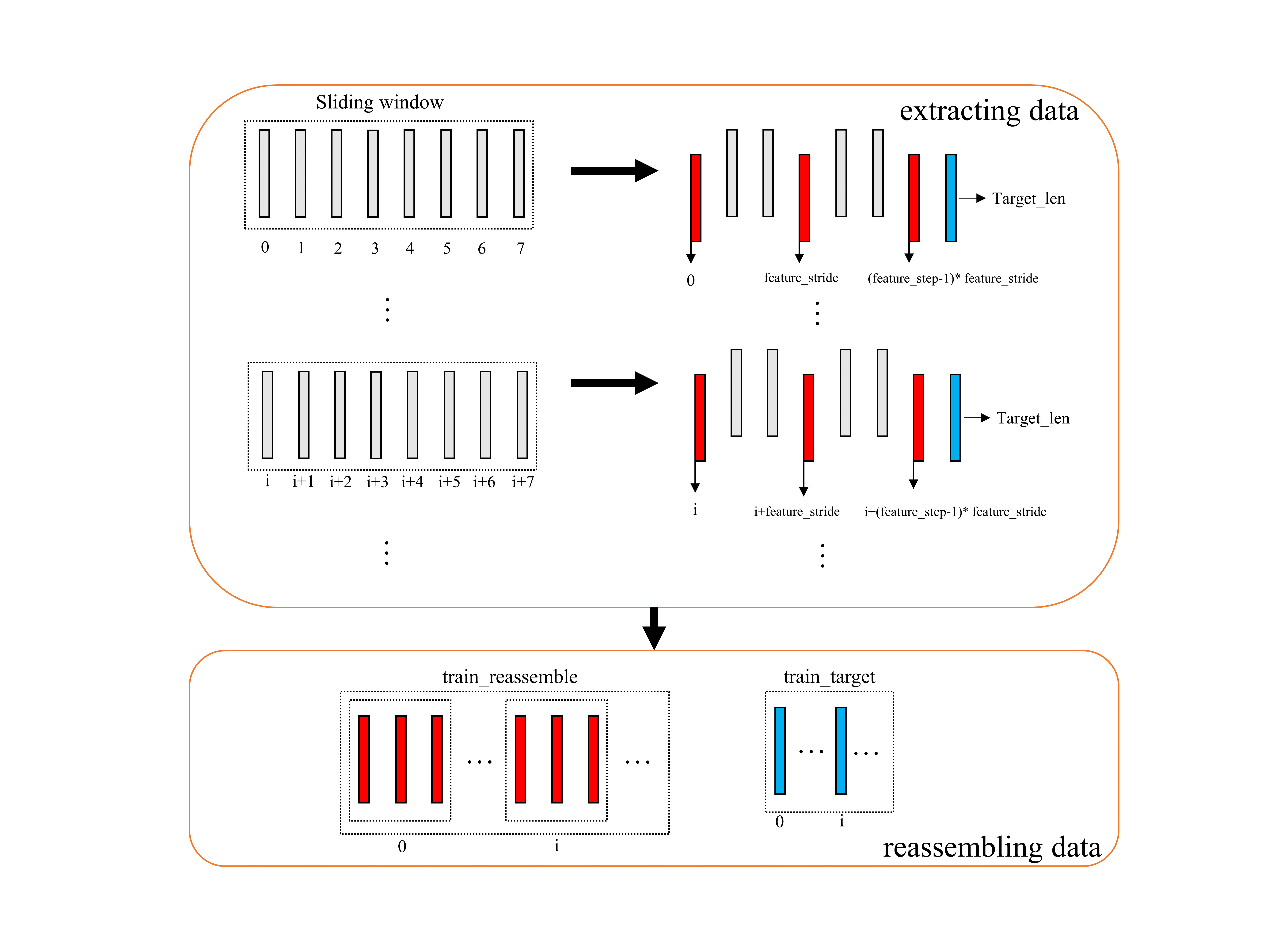
Above is the visualization of a new time series's construction. In this situation, feature_stride = 3(means sampling interval), feature_step = 3(means how many times we sample).Other time series are just the same situation.
Through the process in the figure shown above, we can calculate the length of train_trend is $30844-12247*4=22780$, which is the minimum among three time series.
Operations
- Denormalization/Normalization
- Visualization
- Temporal Knowledge Exploitation
- Spatial knowledge Exploration
- Access to raw data
import matplotlib.pyplot as plt
from UCTB.preprocess.preprocessor import Normalizer
# without normalization
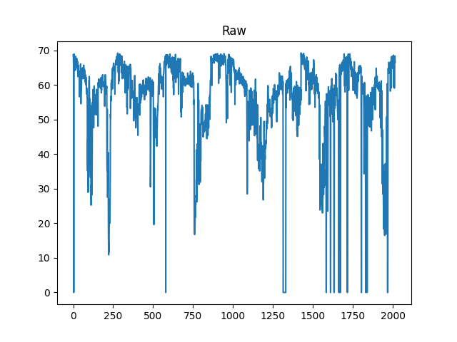
target_node = 5
plt.plot(data_loader.traffic_data[:,5])
plt.title('Raw')
plt.show()
# normalization
normalizer=Normalizer(data_loader.traffic_data)
X_normalized = normalizer.min_max_normal(data_loader.traffic_data)
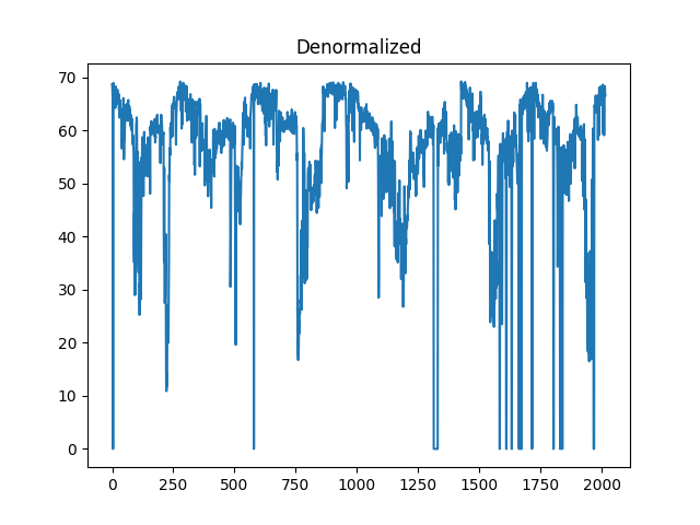
# denormalization
X_denormalized = normalizer.min_max_denormal(X_normalized)
plt.plot(X_normalized[:,5])
plt.title('Normalized')
plt.show()
plt.plot(X_denormalized[:,5])
plt.title('Denormalized')
plt.show()

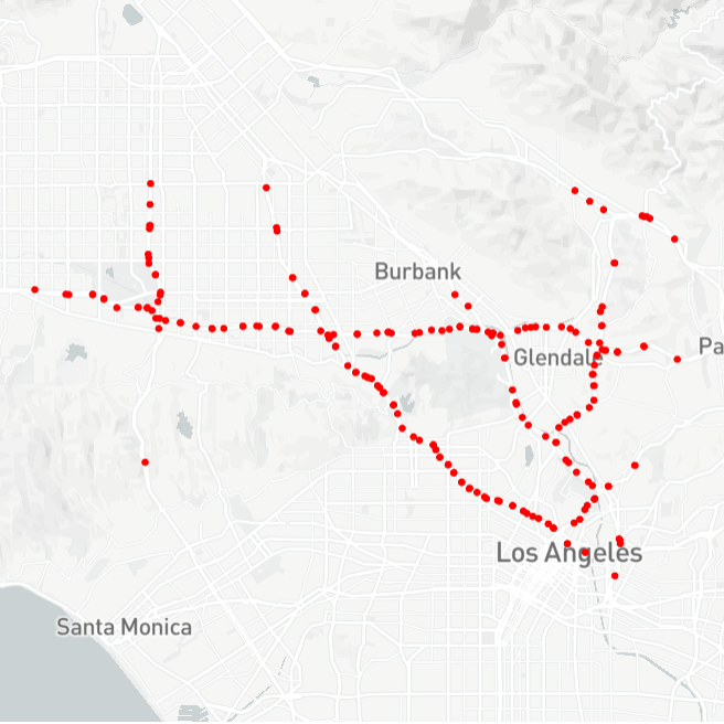
# Nodes' location visualizations
data_loader.st_map()
Visualization result is as follows:
# data visualization
import seaborn as sns
import matplotlib.pyplot as plt
real_denormed=data_loader.normalizer.min_max_denormal(data_loader.test_y)
sns.heatmap(real_denormed[:,:,0], cmap='Reds', vmin = -1000, vmax = 4000)
plt.ylabel("Time Slot")
plt.xlabel("Sensor Node")
plt.title("Visualization")
plt.show()
# Feature stitching
X = data_loader.make_concat()
print('before concatenate')
print('closeness')
print(data_loader.train_closeness.shape)
print('period')
print(data_loader.train_period.shape)
print('trend')
print(data_loader.train_trend.shape)
print('After concatenate')
print(X.shape)
before concatenate
closeness
(22780, 207, 6, 1)
period
(22780, 207, 7, 1)
trend
(22780, 207, 4, 1)
After concatenate
(22780, 207, 17, 1)
# access to raw data
print(data_loader.traffic_data[0,0])
64.375
4.3.2. Model definition, train, test and evaluation
We use XGBoost interface in UCTB as an example to define a model. Since there are total 207 stations in METR_LA dataset, we define 207 XGBoost models respectively. They are trained and tested in their own iteration related to stations. Finally, when we evaluate our model, we consider the prediction results as a whole and evaluate it against GroundTruth provided by data_loader using RMSE metric.
from UCTB.evaluation import metric
from UCTB.model import XGBoost
import UCTB.evaluation.metric as metric
prediction_test = []

for i in range(data_loader.station_number):

    print('*************************************************************')
    print('Station', i)

    model = XGBoost(n_estimators=100, max_depth=3, objective='reg:squarederror')

    model.fit(np.concatenate((data_loader.train_closeness[:, i, :, 0],
                              data_loader.train_period[:, i, :, 0],
                              data_loader.train_trend[:, i, :, 0],), axis=-1),
              data_loader.train_y[:, i, 0])

    p_test = model.predict(np.concatenate((data_loader.test_closeness[:, i, :, 0],
                                           data_loader.test_period[:, i, :, 0],
                                           data_loader.test_trend[:, i, :, 0],), axis=-1))

    prediction_test.append(p_test.reshape([-1, 1, 1]))

prediction_test = np.concatenate(prediction_test, axis=-2)

y_truth = data_loader.normalizer.inverse_transform(data_loader.test_y)
y_pred = data_loader.normalizer.inverse_transform(prediction_test)
y_truth = y_truth.reshape([-1,207])
y_pred = y_pred.reshape([-1,207])
print('Test RMSE', metric.rmse(y_pred, y_truth))
plt.title('XGBoost Result')
plt.xlabel('Time Slot')
plt.ylabel('Speed')
plt.plot(y_pred[:12*24*7,target_node])
plt.plot(y_truth[:12*24*7,target_node])
plt.legend(['gt','pred'])
plt.show()
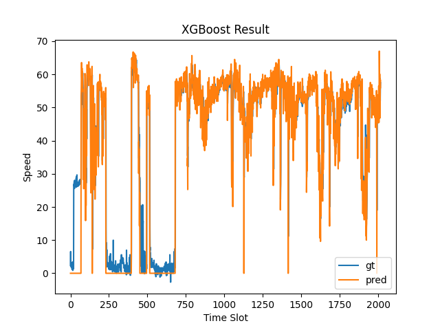
Test RMSE 5.549781682961724
4.3.3. Single vs. Multiple kinds of temporal knowledge
4.3.3.1. Use temporal closeness feature in regression
UCTB provides many classical and popular spatial-temporal predicting models. These models can be used to either predicting series for a single station or all stations. You can find the details in UCTB.model.
The following example shows how to use a XGBoost model to handle a simple time series predicting a problem. We will try to predict the bike demands test_y of a fixed station target_node in New York City by checking back the historical demands in recent time slots train_closeness.
import numpy as np
import matplotlib.pyplot as plt

from UCTB.model import XGBoost
from UCTB.dataset import NodeTrafficLoader
from UCTB.evaluation import metric

target_node = 233
When initializing the loader, we use past 12 time slots (timesteps) of closeness as input, 1 timestep in the next as output and set the timesteps of other features period_len, period_len to zero.
data_loader = NodeTrafficLoader(data_range=0.1, dataset='Bike', city='NYC',
                                closeness_len=12, period_len=0, trend_len=0,
                                target_length=1, test_ratio=0.2,
                                normalize=False, with_lm=False, with_tpe=False)
The well-loaded data contain all 717 stations' data. Therefore it is needed to specify the target station by target_station.
print(data_loader.train_closeness.shape)
print(data_loader.test_closeness.shape)
print(data_loader.test_y.shape)
(2967, 717, 12, 1)
(745, 717, 12, 1)
(745, 717, 1)
train_x, test_x = data_loader.train_closeness[:, target_node, :, 0], data_loader.test_closeness[:, target_node, :, 0]
train_y = data_loader.train_y[:, target_node,0]
test_y = data_loader.test_y[:, target_node, 0]
Inspect the shape of data. Here are the all we need for one-station prediction.
print(train_x.shape)
print(train_y.shape)
print(test_x.shape)
print(test_y.shape)
(2967, 12)
(2967,)
(745, 12)
(745,)
Build the XGBoost model.
model = XGBoost(n_estimators=100, max_depth=3, objective='reg:linear')
Now, we can fit the model with the train dataset and make predictions on the test dataset.
model.fit(x=train_x)
predictions = model.predict(test_x)
We can evaluate the performance of the model by build-in UCTB.evaluation APIs.
test_rmse = metric.rmse(predictions, test_y)
print(test_rmse)
3.6033132
4.3.3.2. Make full use of closeness, period, and trend features
In this case, let's take more temporal knowledge related to target_node into account. We will concatenate factors including closeness, period, and trend, and use XGBoost as the predicting model.
import numpy as np
import matplotlib.pyplot as plt

from UCTB.model import XGBoost
from UCTB.dataset import NodeTrafficLoader
from UCTB.evaluation import metric

target_node = 233

data_loader = NodeTrafficLoader(data_range=0.1, dataset='Bike', city='NYC',
                                closeness_len=6, period_len=7, trend_len=4,
                                target_length=1, test_ratio=0.2,
                                normalize=False, with_lm=False, with_tpe=False)

train_closeness = data_loader.train_closeness[:, target_node, :, 0]
train_period = data_loader.train_period[:, target_nodze, :, 0]
train_trend = data_loader.train_trend[:, target_node, :, 0]
train_y = data_loader.train_y[:, target_node, 0]

test_closeness = data_loader.test_closeness[:, target_node, :, 0]
test_period = data_loader.test_period[:, target_node, :, 0]
test_trend = data_loader.test_trend[:, target_node, :, 0]
test_y = data_loader.test_y[:, target_node, 0]

train_X = np.concatenate([train_closeness, train_period, train_trend], axis=-1)
test_X = np.concatenate([test_closeness, test_period, test_trend], axis=-1)

print(train_X.shape)
print(train_y.shape)
print(test_X.shape)
print(test_y.shape)

model = XGBoost(n_estimators=100, max_depth=3, objective='reg:linear')
model.fit(train_X, train_y)
predictions = model.predict(test_X)
print('Test RMSE', metric.rmse(predictions, test_y))
(2307, 17)
(2307,)
(745, 17)
(745,)
Test RMSE 3.3267457
4.4. Advanced Features
4.4.1. Build your own model using UCTB
UCTB provides extendable APIs to build your own model. Currently, it can support the running of all the 1.x version of Tensorflow-based models. In the following tutorial, we will show you how to takes the least efforts to implement a UCTB model.
Commonly, a new model needs to inherit BaseModel to acquire the features provided by UCTB, such as batch division, early stopping, etc. The necessary components for a subclass of BaseModel include:
self.__init__(). Define the model's parameters related to the architecture. You should call the super class's constructor at first.self.build(). Build the architecture here. You should construct the graph at the beginning of this function and call the super class'sbuild()function at the end.self._input. Thedictused to record the acceptable inputs of the model, whose keys are the parameter names inmodel.fit()andmodel.predict()and values are the name of related tensors.self._output. Thedictused to record the outputs of the model. You should fill the required keyspredictionandlosswith the names of tensors in your case.self._op. Thedictused to define all the operations for the model. Basic usage for it is to record the training operation, for example, the minimizing loss operation of an optimizer. Use keytrain_opto record it.
For more examples, you can refer to the implementations of build-in models in UCTB.model.
from UCTB.model_unit import BaseModel

class MyModel(BaseModel):
    def __init__(self,

                 code_version='0',
                 model_dir='my_model',
                 gpu_device='0',
                ):
        super(MyModel, self).__init__(code_version=code_version,
                                      model_dir=model_dir, gpu_device=gpu_device)
        ...

    def build(self, init_vars=True, max_to_keep=5):
        with self._graph.as_default():
            ...
            self._input['inputs'] = inputs.name
            self._input['targets'] = targets.name

            ...
            self._output['prediction'] = predictions.name
            self._output['loss'] = loss.name
            self._op['train_op'] = train_op.name

        super(MyModel, self).build(init_vars=init_vars, max_to_keep=5)
Next, in a concrete case, we will realize a Long short-term memory (LSTM) model to make the all-station prediction that accepts time series of 717 stations and predict the future of them as a whole.
For the mechanism of LSTM, you can refer to Gers, F. A., Schmidhuber, J., & Cummins, F. (1999). Learning to forget: Continual prediction with LSTM.
import numpy as np
import tensorflow as tf
from UCTB.dataset import NodeTrafficLoader
from UCTB.model_unit import BaseModel
from UCTB.preprocess import SplitData
from UCTB.evaluation import metric
class LSTM(BaseModel):
    def __init__(self,
                 num_stations,
                 num_layers,
                 num_units,
                 input_steps,
                 input_dim,
                 output_steps,
                 output_dim,
                 code_version='0',
                 model_dir='my_lstm',
                 gpu_device='0'):
        super(LSTM, self).__init__(code_version=code_version,
                                   model_dir=model_dir, gpu_device=gpu_device)
        self.num_stations = num_stations
        self.num_layers = num_layers
        self.num_units = num_units
        self.input_steps = input_steps
        self.input_dim = input_dim
        self.output_steps = output_steps
        self.output_dim = output_dim

    def build(self, init_vars=True, max_to_keep=5):
        with self._graph.as_default():
            inputs = tf.placeholder(tf.float32, shape=(None, self.num_stations,
                                                       self.input_steps, self.input_dim))
            targets = tf.placeholder(tf.float32, shape=(None, self.num_stations,
                                                       self.output_steps, self.output_dim))
            # record the inputs of the model
            self._input['inputs'] = inputs.name
            self._input['targets'] = targets.name

            inputs = tf.reshape(inputs, (-1, self.input_steps, self.num_stations*self.input_dim))

            def get_a_cell(num_units):
                lstm = tf.nn.rnn_cell.BasicLSTMCell(num_units, state_is_tuple=True)
                return lstm

            stacked_cells = tf.contrib.rnn.MultiRNNCell([get_a_cell(self.num_units) for _ in range(self.num_layers)], state_is_tuple=True)
            outputs, final_state = tf.nn.dynamic_rnn(stacked_cells, inputs, dtype=tf.float32)

            stacked_outputs = tf.reshape(outputs, shape=(-1, self.num_units*self.input_steps))
            predictions = tf.layers.dense(stacked_outputs, self.output_steps*self.num_stations*self.output_dim)
            predictions = tf.reshape(predictions, shape=(-1, self.num_stations, self.output_steps, self.output_dim))

            loss = tf.sqrt(tf.reduce_mean(tf.square(predictions - targets)))
            train_op = tf.train.AdamOptimizer().minimize(loss)

            # record the outputs and the operation of the model
            self._output['prediction'] = predictions.name
            self._output['loss'] = loss.name
            self._op['train_op'] = train_op.name

        # must call super class' function to build
        super(LSTM, self).build(init_vars=init_vars, max_to_keep=5)
Load the dataset by loader and transform them into the formats your model accepts. If the loader APIs are not filled your demands, you can inherit loader and wrapper it according to your desires (see Quickstart for more details).
data_loader = NodeTrafficLoader(data_range=0.1, dataset='Bike', city='NYC',
                                closeness_len=6, period_len=0, trend_len=0,
                                target_length=1, test_ratio=0.2,
                                normalize=True, with_lm=False, with_tpe=False)
train_y = np.expand_dims(data_loader.train_y, axis=-1)
test_y = np.expand_dims(data_loader.test_y, axis=-1)
model = LSTM(num_stations=data_loader.station_number,
             num_layers=2,
             num_units=512,
             input_steps=6,
             input_dim=1,
             output_steps=1,
             output_dim=1)
model.build()
print(model.trainable_vars)  # count the trainble parameters
6821581
Use your model to training and predicting. model.fit() method presets lots of useful functions, such as batch division and early stopping. Check them in UCTB.model_unit.BaseModel.BaseModel.fit.
model.fit(inputs=data_loader.train_closeness,
          targets=train_y,
          max_epoch=10,
          batch_size=64,
          sequence_length=data_loader.train_sequence_len,
          validate_ratio=0.1)
No model found, start training
Running Operation ('train_op',)
Epoch 0: train_loss 0.016053785 val_loss 0.01606118
Epoch 1: train_loss 0.015499311 val_loss 0.015820855
Epoch 2: train_loss 0.015298592 val_loss 0.015657894
Epoch 3: train_loss 0.015163456 val_loss 0.015559187
Epoch 4: train_loss 0.015066812 val_loss 0.015342651
Epoch 5: train_loss 0.015016247 val_loss 0.015287879
Epoch 6: train_loss 0.014899823 val_loss 0.015249459
Epoch 7: train_loss 0.014773054 val_loss 0.015098239
Epoch 8: train_loss 0.014655286 val_loss 0.015097916
Epoch 9: train_loss 0.014558283 val_loss 0.015108417
predictions = model.predict(inputs=data_loader.test_closeness,
                            sequence_length=data_loader.test_sequence_len)
Reverse the normalization by data_loader and evaluate the results:
predictions = data_loader.normalizer.inverse_transform(predictions['prediction'])
targets = data_loader.normalizer.inverse_transform(test_y)
print('Test result', metric.rmse(prediction=predictions, target=targets))
Test result 2.9765626570592545
Since we only use a short period of the dataset (data_range=0.1) in this toy example, the result looks good compared with the experiment. You can also take a try to test the completed dataset on your model.
4.4.2. Build your own graph with STMeta
Next, we will use the Top-K graph as an example to illustrate how to build customized graphs in UCTB. All of the code in this section can be found here.
Top-K graph
First of all, the customized graphs used in this section is called Top-K graph. We construct the corresponding adjacent graph by marking the point pair that consist of each point and its nearest K points as 1, and the others are marked as 0. Then, we use the adjacent graph to generate the laplacian matrix for input. The hyperparameter K is designed via ad-hoc heuristics. In this demonstration, we chose 23 as the value of K.
Realize TopK graph analysis module
To adopt customized graphs (e.g., Top-K) in UCTB, you should first build your own analysis class by inheriting UCTB.preprocess.GraphGenerator class.
It is worth noting that the ultimate goal is to generate the member variables: self.LM and self.AM, which is the input matrix of the graph. In this phase, we need to make the corresponding analytical implementation according to the type of the custom graph passed in.
# "UCTB/preprocess/topKGraph.py"
import heapq
import numpy as np
from UCTB.preprocess.GraphGenerator import GraphGenerator

# Define the class: topKGraph
class topKGraph(GraphGenerator):  # Init NodeTrafficLoader

   def __init__(self,**kwargs):

       super(topKGraph, self).__init__(**kwargs)

       for graph_name in kwargs['graph'].split('-'):

# As the basic graph is implemented in GraphGenerator, you only need to implement your own graph function instead of the existing one.
           if graph_name.lower() == 'topk':
               lat_lng_list = np.array([[float(e1) for e1 in e[2:4]]
                                        for e in self.dataset.node_station_info])
               # Handling
               AM = self.neighbour_adjacent(lat_lng_list[self.traffic_data_index],
                                       threshold=int(kwargs['threshold_neighbour']))
               LM = self.adjacent_to_laplacian(AM)

               if self.AM.shape[0] == 0:  # Make AM
                   self.AM = np.array([AM], dtype=np.float32)
               else:
                   self.AM = np.vstack((self.AM, (AM[np.newaxis, :])))

               if self.LM.shape[0] == 0:  # Make LM
                   self.LM = np.array([LM], dtype=np.float32)
               else:
                   self.LM = np.vstack((self.LM, (LM[np.newaxis, :])))

# Implement the details of building the Top-K graph.
   def neighbour_adjacent(self, lat_lng_list, threshold):
       adjacent_matrix = np.zeros([len(lat_lng_list), len(lat_lng_list)])
       for i in range(len(lat_lng_list)):
           for j in range(len(lat_lng_list)):
               adjacent_matrix[i][j] = self.haversine(
                   lat_lng_list[i][0], lat_lng_list[i][1], lat_lng_list[j][0], lat_lng_list[j][1])
       dis_matrix = adjacent_matrix.astype(np.float32)

       for i in range(len(dis_matrix)):
           ind = heapq.nlargest(threshold, range(len(dis_matrix[i])), dis_matrix[i].take)
           dis_matrix[i] = np.array([0 for _ in range(len(dis_matrix[i]))])
           dis_matrix[i][ind] = 1
       adjacent_matrix = (adjacent_matrix == 1).astype(np.float32)
       return adjacent_matrix
Redefine the call statement of the above class
# "UCTB/Experiments/CustomizedDemo/STMeta_Obj_topk.py"

# Import the Class: topKGraph
from topKGraph import topKGraph
# Call topKGraph to initialize and generate AM and LM
graphBuilder = topKGraph(graph=args['graph'],
                         data_loader=data_loader,
                         threshold_distance=args['threshold_distance'],
                         threshold_correlation=args['threshold_correlation'],
                         threshold_interaction=args['threshold_interaction'],
                         threshold_neighbour=args['threshold_neighbour'])
# ......
Modify the function call location
Add the new graph name when fitting model and then execute it for experiments. code
os.system('python STMeta_Obj_topk.py -m STMeta_v1.model.yml -d metro_shanghai.data.yml '
          '-p graph:Distance-Correlation-Line-TopK,MergeIndex:12')
We conduct experiments on Metro_Shanghai dataset and use the STMeta_V1 to model both "Distance-Correlation-Line" graph and "Distance-Correlation-Line-TopK" and the results are following:
| Metro: Shanghai | Graph | Test-RMSE |
|---|---|---|
| STMeta_V1 | Distance-Correlation-Line | 153.17 |
| STMeta_V1 | Distance-Correlation-Line-TopK | 140.82 |
The results show that the performance of STMeta_V1 with the graph "Distance-Correlation-Line-TopK" is better than "Distance-Correlation-Line" model and the RMSE is reduced by about 12.4%, which validates the effectiveness of the topk graph for spatiotemporal modeling STMeta algorithm.